A Rube Goldberg machine is a deliberately over-engineered or overdone machine that performs a very simple task in a very complex fashion, usually including a chain reaction[See Ref.: wikipedia]. In this project we have created a simulation of a Rube Goldberg machine we designed, in C++ using the Box2D library. The Rube Goldberg machine's final aim is the task of setting into motion a rocket(an anti-gravity body). We have created a GUI interface for visualization of the simulation and a non-GUI version for analysis of code statistics. We profile the code using gprof, the inbuilt Linux profiling tool, in order to identify which part of the simulation is taking the maximum amount of time to execute. Using this information, we optimize the code. In this report we have given a gist of our design, its salient features and working. Also this report gives the observations on the profiling of the code and the possible optimizations that can be done.
Design of the Simulation
This section explains the original design planned in for the simulation, the final design prepared and the changes done. It reflects on the salient features of Box2D library we have utilized in our simulation and various important elements, which are a part of the simulation. The original design was created at the beginning of the course, when our knowledge of Box2D was much less. Thus the design was rather minimal. However, now that we have got to learn more about Box2D[See Ref.: box2d-guide], we have added a few more elements to the simulation design to make it more interesting.
The Original Planned Design of the Simulation
The Original Planned Design
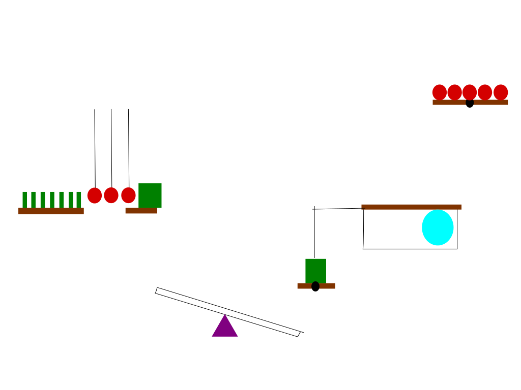
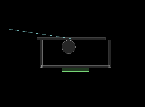
The above image illustrates the original design planned for the simulation. The working of this design is as follows:
A bullet will be fired in the air. In its trajectory, it will hit a stack of dominoes which will topple. This in turn, will oscillate a Newton's pendulum(set of pendulums). The last pendulum will topple a heavy square block on to a seesaw. The other arm of the seesaw will rotate a platform and the weight on the platform will fall down. This weight is connected to the lid of a container with a pulley. While the lid is opened, a balloon in the container will rise, and topple balls into a W shaped pipe.
The Final Simulation Design
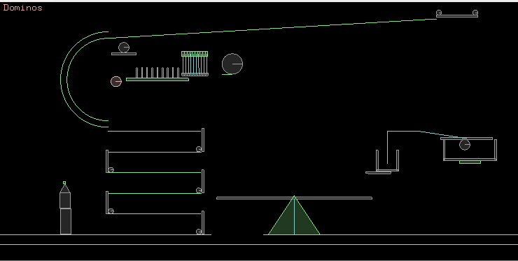
The Final Design
The working of the final design is as follows: A balloon rises and knocks off a ball that falls on the dominoes. The dominoes begin to topple and the last domino pushes the first of a set of Newton's pendulums. The last block topples off a heavy sphere that falls onto the left arm of the see saw wedge. The other arm of the see saw hits a rotating shelf which causes the block on top of it to fall. The block is connected by a pulley to the lid of a container. The lid is opened as the block falls and the balloon in the container rises and hits the platform. This causes one of the two balls to roll onto the sloping surace, through the spherical tube and hit the first of series of vertical shafts. Each of the shafts rotates pushing the next ball to roll and hit the next shaft. The last ball hits the block which is holding the rocket and causes it to "launch" (move upwards very fast).
Key Elements and Features
The important elements in the design of are simulation are:
Newton's Pendulum: The Newton's Pendulums are a set of pendulums placed close to each other, so that when one is made to oscillate it sets into motion all the subsequent pendulums. Each of the pendulum is created using a static box, used for the support and a dynamic body box, which acts as the bob. The two bodies are connected by a revolute joint.
See Saw Arrangement: The heavy sphere see-saw arrangement place in the center on the ground. It consists of a rectangular dynamic box and a triangular static wedge, which are connected by a revolute joint. The heavy sphere falls on one arm of the see saw and it rotates, thereby triggering the pulley system.
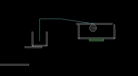
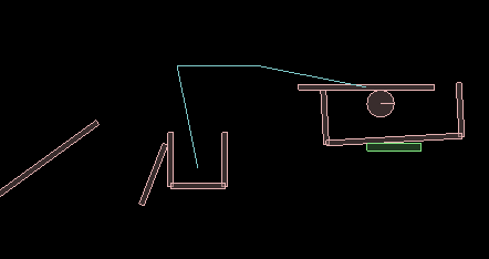
The Pulley System: The pulley system consists of a block and the lid of the container which are connected by a pulley joint hinged at the appropriate places. The see saw topples the support of the block and it begins to fall down pulling along with it the lid of the container. As the container's lid is opened, it frees the balloon to rise.
Pulley System: [1]At Rest and [2]In Motion
The Balloons: We have used two balloons in the design. The first balloon is the initial trigger that begins the chain of events. The second is the one in the container which then topples overa rotating platform and causes the ball on it to move ahead. Both these balloons are Box2D circle bodies, whose gravity has been scaled to a negative value.
The Spherical Tube: The spherical tube is required to change the direction of the ball, without making it lose momentum. The spherical tube is made by two semi-circular edges. Each of the semi-circular edges is itself made by the combination of 45 small straight line edges (each spanning over approx 2degrees). The ball then transfers this momentum to the vertical rotating shafts. The friction of subsequent the horizontal platforms is kept low and the restitution of the shafts is kept high so that the balls continue to transfer the momentum.
The System of the Rotating Flaps: This arrangement serves as a medium of momentum transfer from the top level to the bottom level. At each level, a sphere moves to the other end and hits the edge of the flap. Due to the motion of this flap, on the level below, a sphere is imparted momentum and its moves to the other end of the level and the same process repeats till one of the spheres hits the base of the rocket.
The Rocket-Block Arrangement: The rocket is a combination of two shapes- a box, and a triangle on top of it. The gravity of this body is scaled to a large negative value. Then a tiny fixed (static) wedge is placed right above it to prevent it from flying off before needed. There is a dynamic block placed right below the rocket, such that the top surface of the block touches the bottom surface of the rocket body. The friction between these two surfaces is set very high and the density of the (dynamic) block is kept low. When the rolling ball hits the block, it moves slightly and due to the friction, the rocket also get enough torque for its center of gravity to be slightly deviated from the the fixed wedge on top. Thus the rocket flies off rapidly.
The salient features of our simulation design which makes it unique would be as follows:
Use of the SetGravityScale(..) function: We have used the SetGravityScale(float) function of Box2D's b2Body class. Using the function we can scale the gravity of any particular body to avalue of our choice. This is used to create objects like the balloons and the rocket. For the balloons, the gravity is scaled by -0.2 and -0.1 respectively, while for the rocket body, the gravity is scaled by a factor of -10.0. The low negative scale for the balloons make them seem to be rising with less acceleration like actual balloons would. The rocket is given highly negative gravity scale so that when set into motion, it rapidly rises giving the feeling that it has been launched!
Scaling Gravity: The ballons and the rocket
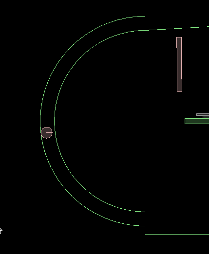
Making the Spherical Tube: The spherical tube was necessary in order to change the direction of the moving ball and to make sure it does not lose its momentum. Using any other mechanical device like a rotating shaft would cause loss in speed. We then decided to create a circular path, so that the direction is changed with as less loss of momentum as possible. Each of the semi-circular edge contains 90 small straight line segments. The circle is divided into 90 segments or arcs of 2 degrees each and each line segment connects the ends of these arcs. These line segments are iteratively create and help to approximate the circle.
The Circular Tube
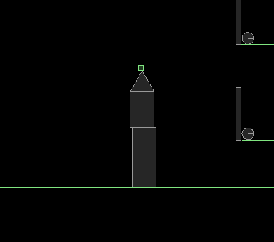
The arrangement to hold and launch the rocket: We decided that we would have a rocket fly off in the end, by making the gravity scaled to a high negative value (-10.0). We kept a small wedge just above the tip of the rocket to prevent it from flying when not needed. There is a dynamic block placed right below the rocket, such that the top surface of the block touches the bottom surface of the rocket body. The friction between these two surfaces is set very high and the density of the (dynamic) block is kept low. When the ball hits the lower block, its low density ensures that it moves a little despite the friction. As it moves it applies friction on the bottom surface of the rocket, thereby providing it enough torque to set it in motion.
The Rocket Arrangement
Timing Plots and Analysis
We created and analyzed the timimg plots of the various times for the execution using matplotlib plotting module in Python[See Ref.: matplotlib-guide]. The first step involved generating data of average time required for step , collision , velocity updates and position updates for number of iterations from 1 to 100. For each iteration number, 100 values were generated by running the script 100 times. Then we created various plots of various computational times and analyzed each of the graph plots.
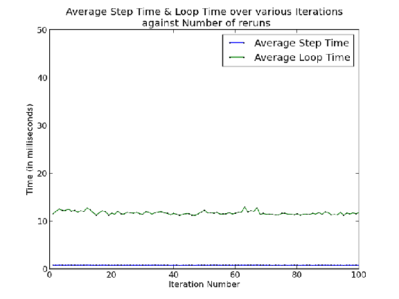
Plot 01: Average Step Time and Average Loop Time v/s Iteration Values
This graph plots Step Time and Loop Time averaged over all reruns against the iteration number. The step time decreases with the number of iterations. This can be attributed to the fact that as the number of iterations increase, the number of computations may be reduced due to the fact that certain computations may not be needed for certain iterations. The loop time increases with iterations which is quite obvious more iterations would naturally mean more time taken for the entire loop. The product of step time and iteration number is approximately equal to the loop time. This is consistent and establishes the fact that the gettimeofday() and b2Timer profile give similar results.
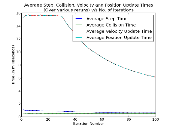
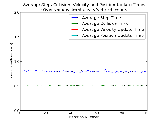
Plot 02: Average Collision Time , Velocity and Position Updates v/s Iteration Values
In the start of the simulation, we can observe that step time remains constant and after nearly 40 iterations, it decreases. This can be attributed to the fact that at the start of the simulation, there are a lot of moving elements (the Dominoes and the Newton's Pendulum). Due to this, step time remains high in the start.
Morover, each of the collision time, velocity update time and position update time show decreasing trends with the iteration value. This trend is similar to that of the average step time. The sum of the collision time, velocity update time and position update time is less than the step time. This is quite natural as there are other event computations in the simulation besides collision, velocity and position computations.
Plot 03: Average Step Time and Average Loop Time v/s Rerun Values
Plotting the step and loop times over rerun number just gives a larger sample over time. This obviously does not affect the trend of the times. The plots for the step and loop times is thus almost constant with slight deviations from the average. For a loaded system the plot pattern remains the same but is just scaled along the Y direction. The graph trends and inferences are similar, but the actual values for the step and loop times are higher. Also the deviations are more, due to more randomness in allocation of resources as many processes are running.
Plot 04: Average Collision Time, Velocity and Position Updates v/s Iteration Values
The analysis of this plot is quite similar to the previous. Again the plots of various event computation times over rerun number just gives a sampling over time and it will not affect the value of the times. The plots for each of the times, is again constant with slight deviations or variations from the average values. For a loaded system, just like the previous plot, trends and inferences are similar, but the actual values for the times are higher.
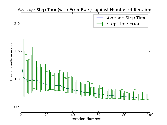
Plot 05: Step Time (with Y Error-Bars) v/s Iteration Values
The trend in the step time is decreasing with the number as interations, in accordance with the first plot. The error bars are larger for lower iteration numbers. This is because with lesser iterations, there is more randomness. Also though the absolute error is very high for lower values of iterations, the relative error is not `very high'. The relative error for lower iteration numbers is, more or less, of the same range as that of the higher iteration numbers. The errors in the step time reduce with the iteration number, with a few anomalies or deviations for certain executions.
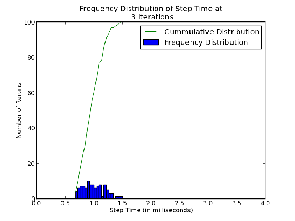
Plot 06: Step Time Frequency and Cumulative Frequency (for n = 3 iterations)
The frequency distibution is more or less uniform with a fairly large value around the average step time over all iterations. It very closely resembles the normal bell curve distribution. Since most values lie within a small range the frequency for that range is significnatly higher than for the other ranges. Thus the cummulative frequency rises steadily in the beginning and the increases steeply near the average time value and again become steady. When the system is loaded, the frequency plot is more distributed, closer to the normal Bell distribution. This is because the deviation in times is larger when the system is loaded as inferred in the previous plot.
Code Profiling and Optimizations
Code Profiles
We profile the code with the profiler gprof and try to draw conclusions on the parts of the code that consume the most amount of time and calls. We have also figured out optimizations that can be carried out to improve the running time for the execution. We compile the code in debug and release verions (i.e. without or with -O3 flags) and examine the difference in profile outputs.
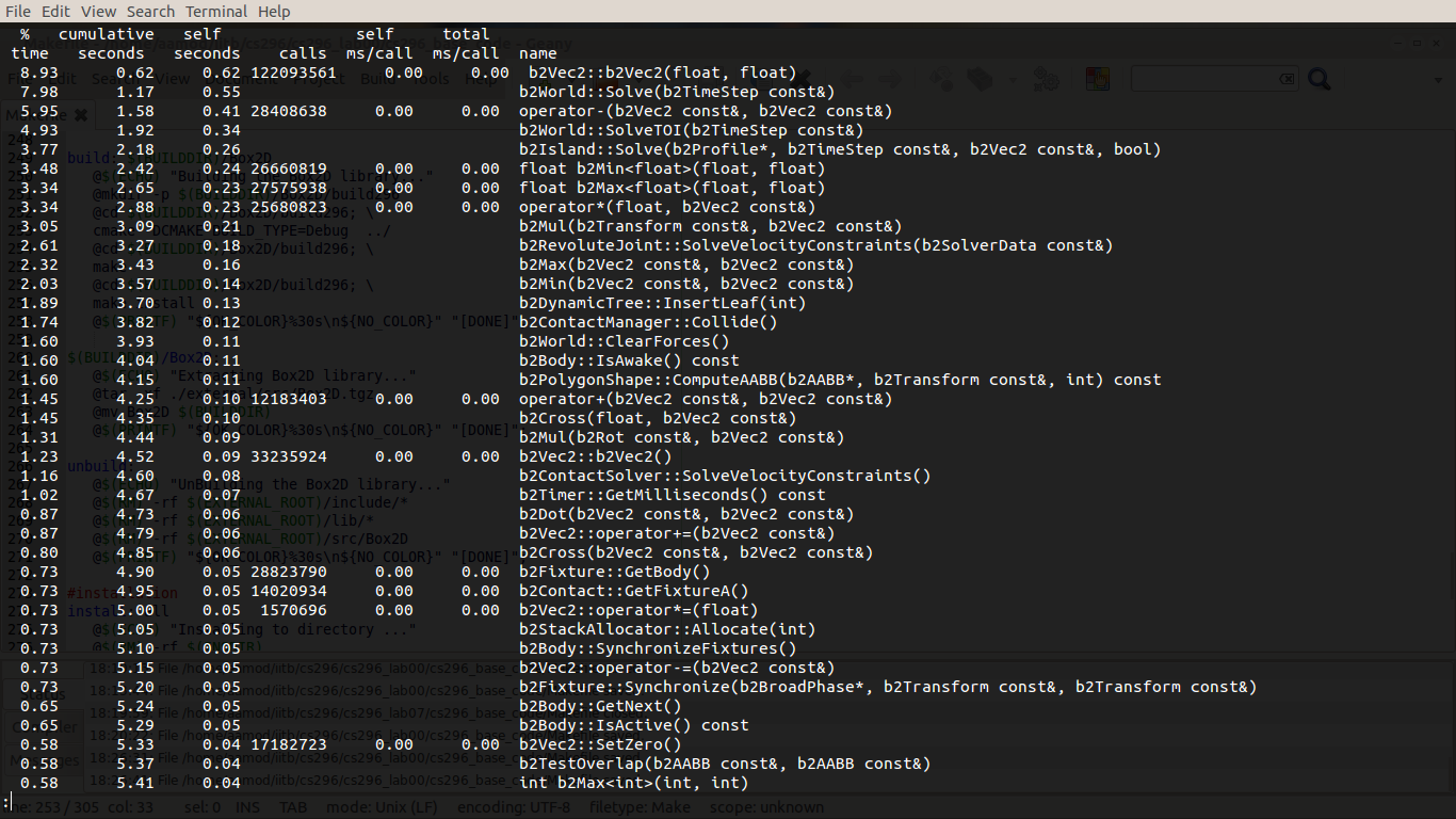
Profiling Output for Debug Version
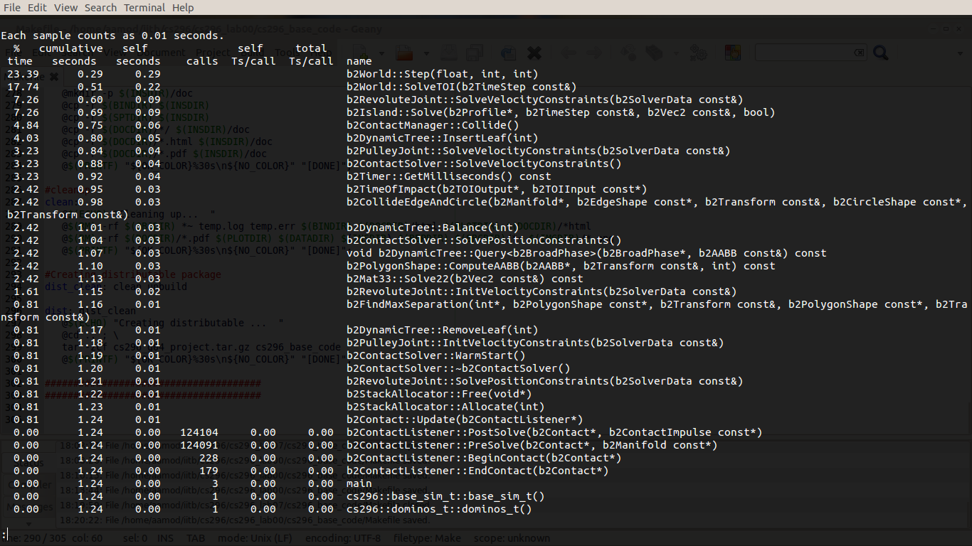
Profiling Output for Release Version
Optimizations
We now list some optimiztions that can be carried to improve the code:
b2ContactSolver::SolveVelocityConstraints()
Debug Time: 0.15; Release Time: 0.04
b2ContactSolver::InitializeVelocityConstraints()
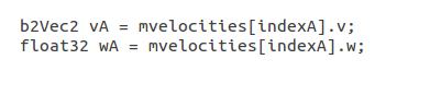
Debug Time: 0.08; Release Time: 0.01 Calling the same array element twice instead of saving it in a temp variable.
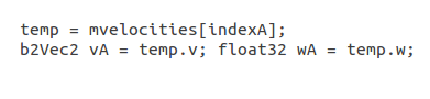
Can be Optimised by,
The Flag -fprefetch-loop-arrays (generate instructions to prefetch memory to improve the performance of loops that access large arrays.) and -fpredictive-commoning (from -O3) optimises this part of the code[See Ref.: gcc-compiler].
float b2Max(float, float) : Time:0.24, Calls:27575938 These overloaded operators perform operations on the vectors. Since,they are called a large amount of times, and each function call adds to the program time, as the program has to remember the program environment and pass the parameters by reference. Due to the large amount of calls, this adds up to significant time in the debug version.
In the release version, these operators are totally eliminated as they are converted to inline functions by the -finline-functions flag[See Ref.: gcc-optimizations] (The compiler heuristically decides which functions are worth integrating in this way). Inline functions are implemented by copying the code in the function itself. This reduces the time of passing the parameters and reduces the overall time of the program.
Debug version:
b2Vec2::b2Vec2(): Calls:122093561
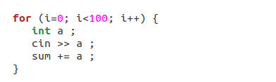
The number of calls to the b2Vec2 constructor is huge because this constructor is called everytime in the loop of SolveVelocityConstraints(). This can be optimised by defining the b2Vec2 ouside the loop. For example:
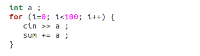
This defines the integer variable a100 times(the variable is assigned memory 100 times) so takes up a lot of time. This can be optimised by defining a outside the loop.
The release version performs this optimization. The number of calls of b2Vec2 constructor is reduced expotentially from 122093561 to 4510 in the release version by defining the vectors outside the loop. This optimises a large amount of memory and time. This optimisation is also applied to b2World::SolveTOI():
Debug Time: 0.34; Release Time: 0.22
Call Graphs
Call graphs are a way of analysing the function calls in the program. Call graphs show the call of functions in a function in the form of a graph. The children functions of a node are called in the function itself. Debug Version:
A Part of the Call Graph for the Debug Version
We can see the many of the functions have children functions: operator*(float, b2Vec2 const\&) etc. These functions call the b2Vec2() constructor(at depth 3 of the tree).
Release Version :
A Part of the Call Graph for the Release Version
As per the inline function optimisation, we can observe that the number of children of the functions have reduced to nearly zero as the children functions are converted to inline functions.